Hist1d.plot() and Hist2d.plot()#
Default plotting methods#
Hist1d and Hist2d provide methods for basic plotting, as
showcased by the following examples:
import matplotlib.pyplot as plt
import atompy as ap
plt.style.use("atom")
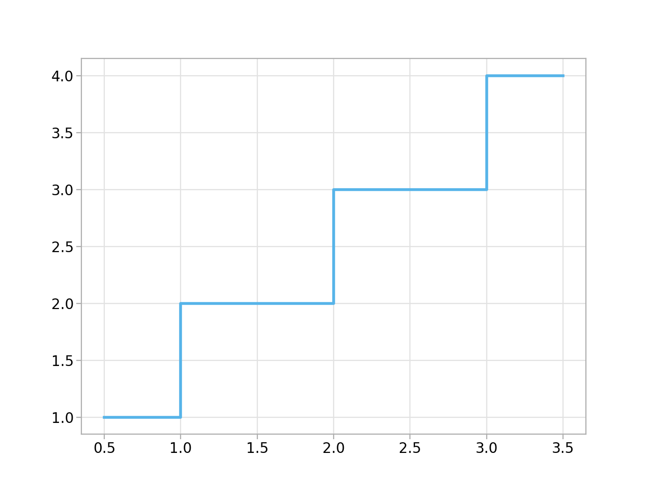
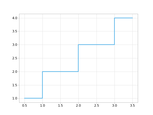
hist = ap.Hist1d((1, 2, 3, 4), (0, 1, 2, 3, 4))
hist.plot(drawstyle="steps-mid")
(Source code, png, hires.png, pdf)
import matplotlib.pyplot as plt
import atompy as ap
plt.style.use("atom")
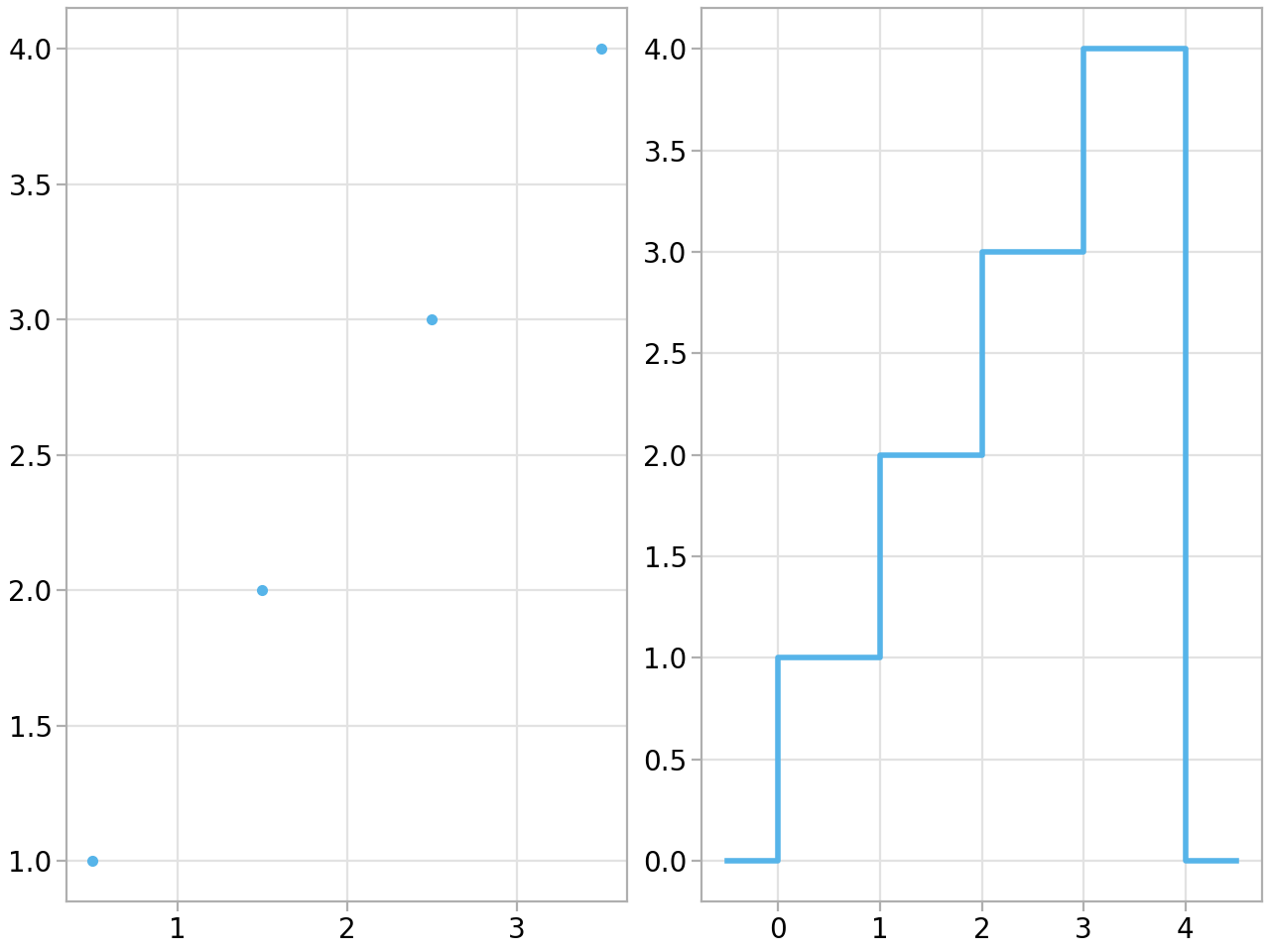
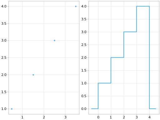
hist = ap.Hist1d((1, 2, 3, 4), (0, 1, 2, 3, 4))
_, axs = plt.subplots(1, 2, layout="compressed")
hist.plot(axs[0], plot_fmt="o")
hist.pad_with(0).plot(axs[1], drawstyle="steps-mid")
plt.show()
(Source code, png, hires.png, pdf)
import matplotlib.pyplot as plt
import numpy as np
import atompy as ap
plt.style.use("atom")
rng = np.random.default_rng(42)
lim = (-2, 2)
size = 1_000
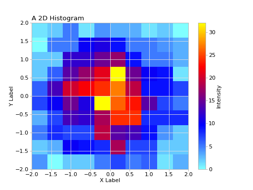
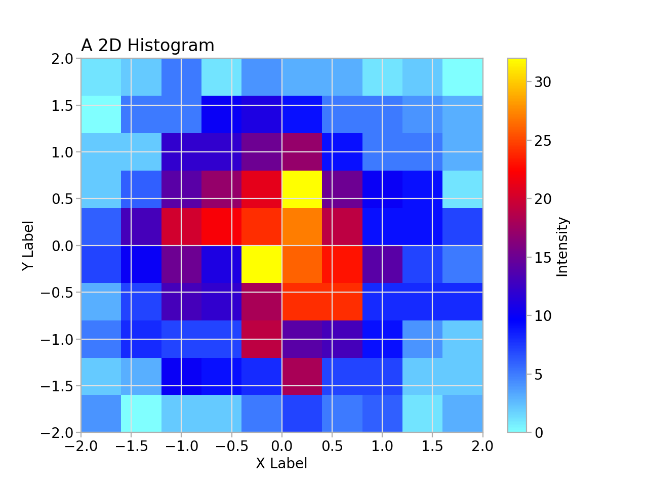
hist = ap.Hist2d(
*np.histogram2d(*rng.normal(size=(2, size)), range=(lim, lim)),
title="A 2D Histogram",
xlabel="X Label",
ylabel="Y Label",
zlabel="Intensity",
)
fig, ax, cb = hist.plot()
plt.show()
(Source code, png, hires.png, pdf)

import matplotlib.pyplot as plt
import numpy as np
import atompy as ap
plt.style.use("atom")
rng = np.random.default_rng(42)
lim = (-2, 2)
size = 1_000
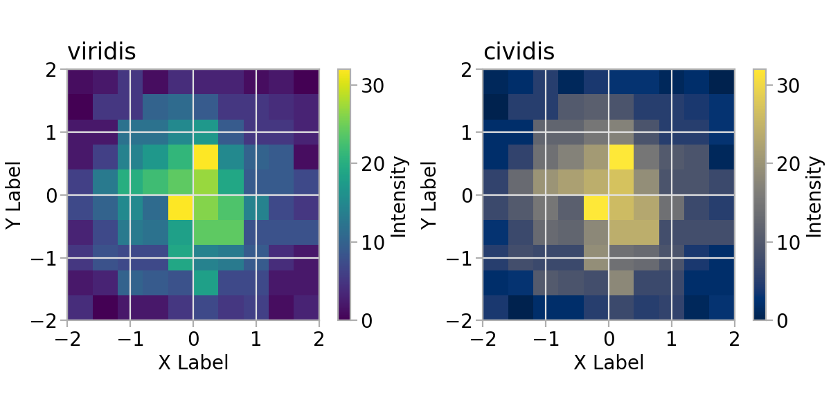
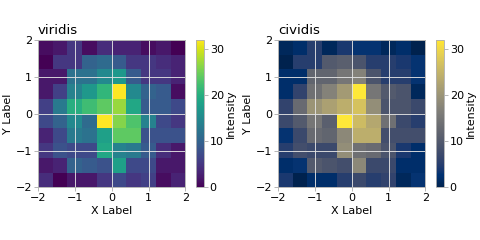
hist = ap.Hist2d(
*np.histogram2d(*rng.normal(size=(2, size)), range=(lim, lim)),
xlabel="X Label",
ylabel="Y Label",
zlabel="Intensity",
)
fig, axs = plt.subplots(ncols=2, layout="compressed", figsize=(6.0, 3.0))
cmaps = "viridis", "cividis"
for ax, cmap in zip(axs, cmaps):
ax.set_box_aspect(1)
hist.plot(ax=ax, title=cmap, cmap=cmap)
(Source code, png, hires.png, pdf)
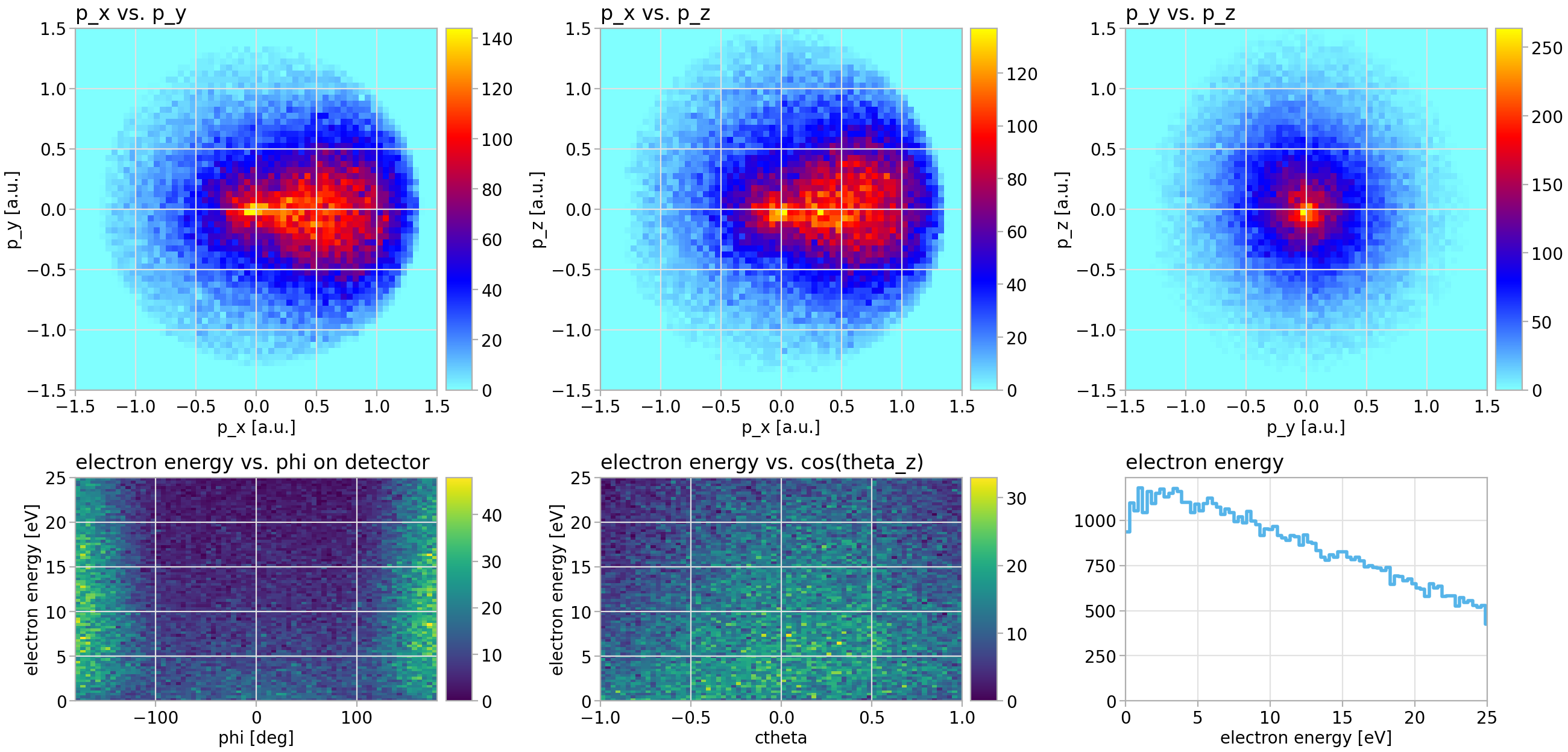
Custom plotting methods#
It is possible to create a derived class inheriting from Hist1d or
Hist2d, and implementing a custom plotting methods for these.
The following example showcases the perks of this approach. Note that the plotting
method uses a custom layout engine (similar to tight_layout())
provided by mplutils.
import matplotlib.pyplot as plt
import mplutils as mplu

import atompy as ap

MAX_ENERGY = 25.0
MAX_MOMENTUM = 1.5


class EnergyHist1d(ap.Hist1d):
    def plot(self, ax):
        fig, ax = super().plot_step(ax=ax, start_at="auto")
        fig.set_layout_engine(mplu.FixedLayoutEngine())
        mplu.set_axes_size(3, aspect=1.0 / 1.618, ax=ax, anchor="W")
        ax.set_ylim(bottom=0)
        ax.set_xlim(self.limits[0], MAX_ENERGY)
        return fig, ax


class EnergyVsAngleHist(ap.Hist2d):
    def plot(self, ax):
        fig, ax, _ = super().plot(ax=ax, cmap="viridis")
        fig.set_layout_engine(mplu.FixedLayoutEngine())
        mplu.set_axes_size(3, aspect=1.0 / 1.618, ax=ax, anchor="W")
        ax.set_ylim(0, MAX_ENERGY)
        return fig, ax


class MomentumMap(ap.Hist2d):
    def plot(self, ax):
        fig, ax, _ = super().plot(ax=ax, cmap="atom")
        fig.set_layout_engine(mplu.FixedLayoutEngine())
        mplu.set_axes_size(3, ax=ax, anchor="W")
        ax.set_xlim(-MAX_MOMENTUM, MAX_MOMENTUM)
        ax.set_ylim(-MAX_MOMENTUM, MAX_MOMENTUM)
        return fig, ax


histos = []
fname = "example.root"

base = "He_Compton/electrons/momenta"
histos.append(MomentumMap.from_root(fname, f"{base}/px_vs_py"))
histos.append(MomentumMap.from_root(fname, f"{base}/px_vs_pz"))
histos.append(MomentumMap.from_root(fname, f"{base}/py_vs_pz"))
base = "He_Compton/electrons/energy"
histos.append(EnergyVsAngleHist.from_root(fname, f"{base}/phi_vs_electron_energy"))
histos.append(EnergyVsAngleHist.from_root(fname, f"{base}/ctheta_vs_electron_energy"))
histos.append(EnergyHist1d.from_root(fname, f"{base}/electron_energy"))

plt.style.use("atom")
fig, axs = plt.subplots(2, 3)

for histo, ax in zip(histos, axs.flat):
    histo.plot(ax)
(Source code, png, hires.png, pdf)
