profile_along_y#
- Hist2d.profile_along_y(option='')[source]#
Get the y-profile.
Calculate the mean value and its error per row. Which type of error is controled with option.
- Parameters:
- option“”, “s”, “i”, or “g”, default “”
Control type of errors, see Notes.
“”: Error of the mean of all Y values
“s”: Standard deviation of all Y
“i”: See Notes
“g”: Error of a weighted mean for combining measurements with variances of \(w\).
- Returns:
Notes
See TProfile of the ROOT Data Analysis Framework.
For a histogram \(X\) vs \(Y\), the following is calculated for each \(Y\) value.
\[\begin{split}H(j) &= \sum w X \\ E(j) &= \sum w X^2 \\ W(j) &= \sum w \\ h(j) &= H(j) / W(j) \\ s(j) &= \sqrt{E(j) / W(j) - h(j)^2} \\ e(j) &= s(j) / \sqrt{W(j)}\end{split}\]Here, \(w\) are the counts of bin j.
Examples
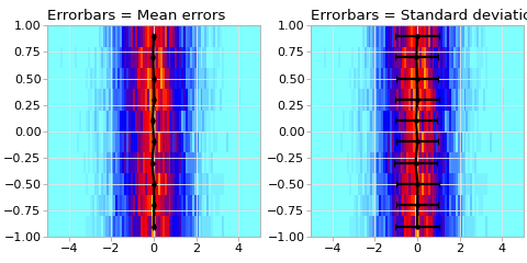
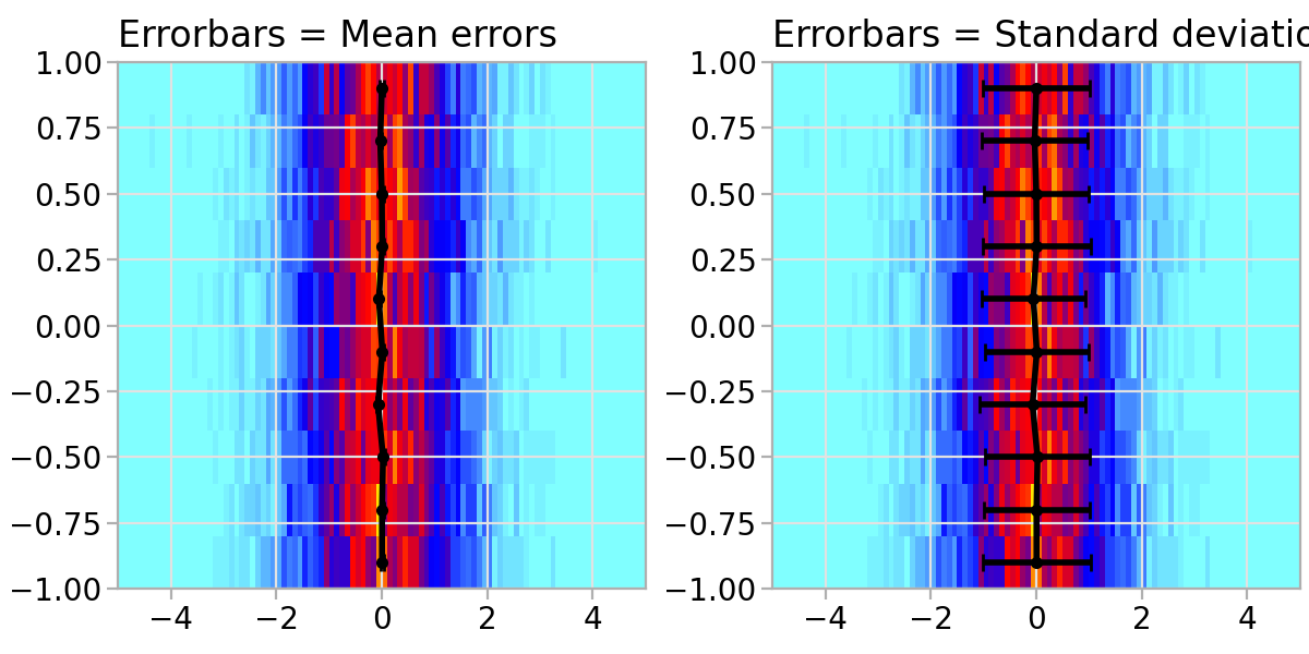
import matplotlib.pyplot as plt
import numpy as np

import atompy as ap

plt.style.use("atom")

# get some random data
gen = np.random.default_rng(42)
x_sample = gen.normal(size=10_000)
y_sample = gen.uniform(-1, 1, size=10_000)

# create a histogram
hist = ap.Hist2d(
    *np.histogram2d(x_sample, y_sample, bins=(100, 10), range=((-5, 5), (-1, 1)))
)
mean, mean_errors = hist.profile_along_y()
_, standard_deviation = hist.profile_along_y("s")

_, axs = plt.subplots(1, 2, layout="compressed", figsize=(6.0, 3.0))
for ax in axs.flat:
    ax.set_box_aspect(1)
    ax.pcolormesh(*hist.for_pcolormesh())

kwargs = dict(fmt="o-", color="k")

axs[0].errorbar(mean, hist.ycenters, xerr=mean_errors, **kwargs)
axs[0].set_title("Errorbars = Mean errors")

axs[1].errorbar(mean, hist.ycenters, xerr=standard_deviation, **kwargs)
axs[1].set_title("Errorbars = Standard deviation")
(
Source code,png,hires.png,pdf)